Guidelines to run the Average rank method over BENGI for GM12878¶

Prerequisites¶

Step 1: run Distance method¶

Step 2: run DNase-expression correlation method¶

Partial reimplementation of `Run-Average-Rank.sh`¶

We replaced the content of local_Scripts/Unsupervised-Methods/Run-Average-Rank.sh with the following:

#!/bin/bash

data=$1
version=$2

# Inserm computer
#workDir=~/Documents
# Personal computer
#workDir=~/Documents/INSERM
# Genotoul
workDir=/work2/project/regenet/workspace/thoellinger

distance=$workDir/BENGI/Distance-Method/Results/$data-Distance.$version.txt
correlation=$workDir/BENGI/Correlation-Methods/Sheffield/Results/$data-Correlation.$version.txt

output_dir=$workDir/BENGI/Correlation-Methods/Average-Rank
mkdir -p $output_dir

# for old format of distance method resulting files (with 2 columns),
# with "." as local decimal separator in bash, use:
#paste $distance $correlation | awk '{print $1 "\t" $2 "\t" $4}' | \
#    sort -k2,2gr | awk 'BEGIN{x=0;r=0}{if (x != $2) r +=1; print $0 \
#    "\t" r; x=$2}' | sort -k3,3gr | awk 'BEGIN{x=0;r=0}{if (x != $3) \
#    r +=1; print $0 "\t" r "\t" ($NF+r)/2; x=$3}' | sort -k6,6g | \
#    awk '{print $1 "\t" 1/$6 "\t" $2 "\t" $3 "\t" $4 "\t" $5 "\t" $6}' > $output_dir/$data-Average-Rank.$version.txt

# for new format of distance method resulting files (with 4 columns), use:

# if the local decimal separator in bash is "," (personal computer, genotoul, ...)
paste $distance $correlation |awk '{print $1 "\t" $2 "\t" $6}' |tr . , | \
    sort -k2,2gr | awk 'BEGIN{x=0;r=0}{if (x != $2) r +=1; print $0 \
    "\t" r; x=$2}' | sort -k3,3gr | awk 'BEGIN{x=0;r=0}{if (x != $3) \
    r +=1; print $0 "\t" r "\t" ($NF+r)/2; x=$3}' | sort -k6,6g | \
    awk '{print $1 "\t" 1/$6 "\t" $2 "\t" $3 "\t" $4 "\t" $5 "\t" $6}' |tr , . > $output_dir/$data-Average-Rank.$version.txt

# if the local decimal separator in bash is ".":
#paste $distance $correlation | awk '{print $1 "\t" $2 "\t" $6}' | \
#    sort -k2,2gr | awk 'BEGIN{x=0;r=0}{if (x != $2) r +=1; print $0 \
#    "\t" r; x=$2}' | sort -k3,3gr | awk 'BEGIN{x=0;r=0}{if (x != $3) \
#    r +=1; print $0 "\t" r "\t" ($NF+r)/2; x=$3}' | sort -k6,6g | \
#    awk '{print $1 "\t" 1/$6 "\t" $2 "\t" $3 "\t" $4 "\t" $5 "\t" $6}' > $output_dir/$data-Average-Rank.$version.txt

Note that we replaced

sort -k3,3gr | awk 'BEGIN{x=0;r=0}{if (x != $2) \
    r +=1; print $0 "\t" r "\t" ($NF+r)/2; x=$2}'

which seems to be an error, with

sort -k3,3gr | awk 'BEGIN{x=0;r=0}{if (x != $3) \
    r +=1; print $0 "\t" r "\t" ($NF+r)/2; x=$3}'

The reason is that the code does as follows:

first, distance and correlation results (which are assumed sorted the very same way - which is the case if they were computed using the dedicated guides mentioned in the prerequisites) are merged
then, the ranks of inverse distances are computed (the smaller the distance, the smaller the rank) with sort -k2,2gr | awk 'BEGIN{x=0;r=0}{if (x != $2) r +=1; print $0 "\t" r; x=$2}'. So the condition on x=$2 ($2 being the inverse distance) ensures the rank remains the same when consecutive inverse distances are constant.
then, the rank of the DNase-expression correlation method, plus the average distance-correlation rank, are computed (the greater the correlation, the smaller the rank) with sort -k3,3gr | awk 'BEGIN{x=0;r=0}{if (x != $3) r +=1; print $0 "\t" r "\t" ($NF+r)/2; x=$3}'. So a condition on $2 (value of the inverse distance) instead of $3 (the correlation) would not make sense.

In the analysis, we will see that using $2 as Moore et al, leads to the very same results (AUPR of predictions over the 6 BENGI for GM12878) as in their paper ; and using $3, which we think is the correct way to do ; gives similar but slightly better results!

One should also note that we added tr . , at the beginning of the code and tr , . at the end. This is needed on every computer where bash default decimal separator is "," instead of ".".

At the end of the day, the fields are as follows:

interaction (ground truth)
final score = 1 / (average rank), such that the smaller the rank, the greater the score (=> high score = interaction suspected)
inverse distance
DNase-expression correlation
inverse distance rank (the smaller the distance, the smaller the rank)
DNase-expression correlation rank (the greater the correlation, the smaller the rank)
average rank (= 1 over final score)

Running the code for BENGI benchmarks over GM12878¶

If working on Genotoul:

conda activate base && conda activate abcmodel && conda activate py2 && module load bioinfo/bedtools-2.27.1

srun --pty bash

Now:

./local_Scripts/Unsupervised-Methods/Run-Average-Rank.sh GM12878.CHiC v3

./local_Scripts/Unsupervised-Methods/Run-Average-Rank.sh GM12878.CTCF-ChIAPET v3

etc

Analysis with R¶

Code¶

.badCode {
background-color: #C9DDE4;
}

library(knitr)
## Global options
options(max.print="75")
opts_chunk$set(echo=TRUE,
                 cache=FALSE,
               prompt=FALSE,
               tidy=TRUE,
               comment=NA,
               message=FALSE,
               warning=FALSE,
               class.source="badCode")
opts_knit$set(width=75)

library(ggplot2)
library(ggpubr) # for ggarrange
library(dplyr) # for bind_rows

# Tools for precision-recall : (see https://classeval.wordpress.com/tools-for-roc-and-precision-recall/)
library(precrec)
#library(ROCR)
#library(pROC)
#library(PRROC)

rm(list = ls())

# Personal
work_dir = "~/Documents/INSERM/"
# Inserm
#work_dir = "~/Documents/"

path_to_results = paste(work_dir, "BENGI/Correlation-Methods/Average-Rank/", sep='')
file_names = c("GM12878.CHiC-Average-Rank.v3.txt", "GM12878.CTCF-ChIAPET-Average-Rank.v3.txt", "GM12878.GEUVADIS-Average-Rank.v3.txt", "GM12878.GTEx-Average-Rank.v3.txt", "GM12878.HiC-Average-Rank.v3.txt", "GM12878.RNAPII-ChIAPET-Average-Rank.v3.txt")
short_names = c('CHiC', 'CTCF', 'GEUVAVDIS', 'GTEx', 'HiC', 'RNAPII')

nb_files = length(file_names)

colnames <- c('interaction', 'score', 'inverse.distance', 'correlation', 'inverse.distance.rank', 'correlation.rank', 'average.rank')
results <- sapply(file_names, simplify=FALSE, function(file_name){
  Df <- read.table(paste(path_to_results, as.character(file_name), sep=''), sep='\t')
  Df[[1]] <- factor(Df[[1]], levels=c(0,1), labels=c("no interaction", "interaction"))
  names(Df) <- colnames
  return(Df)
})
names(results) <- short_names

#library(dplyr)
All_results <- bind_rows(results, .id = 'method') # requires library(dplyr)

str(results)
summary(results$CHiC)

ggplot(aes(y = average.rank, x = method, fill = interaction), data = All_results) + geom_boxplot()

sscurves_avg_rank <- list()s
sscurves_avg_rank <- sapply(results, simplify=FALSE, function(Df){
  evalmod(scores = Df$score, labels = Df$interaction) # comes with "precrec" library
})

#library(ggplot2)
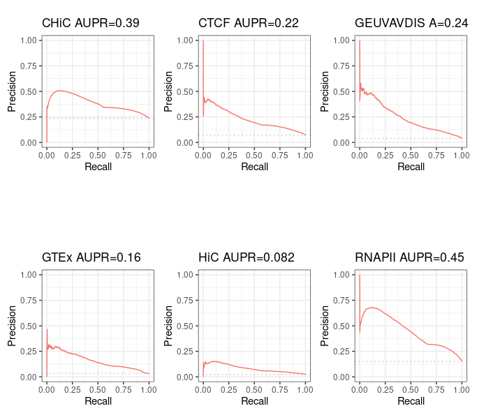
p1 <- autoplot(sscurves_avg_rank[[1]], curvetype = c("PRC")) + ggtitle(paste(short_names[1], signif(attr(sscurves_avg_rank[[1]], 'auc')[[4]][2], digits=2), sep = " AUPR="))
p2 <- autoplot(sscurves_avg_rank[[2]], curvetype = c("PRC")) + ggtitle(paste(short_names[2], signif(attr(sscurves_avg_rank[[2]], 'auc')[[4]][2], digits=2), sep = " AUPR="))
p3 <- autoplot(sscurves_avg_rank[[3]], curvetype = c("PRC")) + ggtitle(paste(short_names[3], signif(attr(sscurves_avg_rank[[3]], 'auc')[[4]][2], digits=2), sep = " A="))
p4 <- autoplot(sscurves_avg_rank[[4]], curvetype = c("PRC")) + ggtitle(paste(short_names[4], signif(attr(sscurves_avg_rank[[4]], 'auc')[[4]][2], digits=2), sep = " AUPR="))
p5 <- autoplot(sscurves_avg_rank[[5]], curvetype = c("PRC")) + ggtitle(paste(short_names[5], signif(attr(sscurves_avg_rank[[5]], 'auc')[[4]][2], digits=2), sep = " AUPR="))
p6 <- autoplot(sscurves_avg_rank[[6]], curvetype = c("PRC")) + ggtitle(paste(short_names[6], signif(attr(sscurves_avg_rank[[6]], 'auc')[[4]][2], digits=2), sep = " AUPR="))

# ggarrange comes with library('ggpubr')
figure <- ggarrange(p1, p2, p3, p4, p5, p6,
                    ncol = 3, nrow = 2)
figure

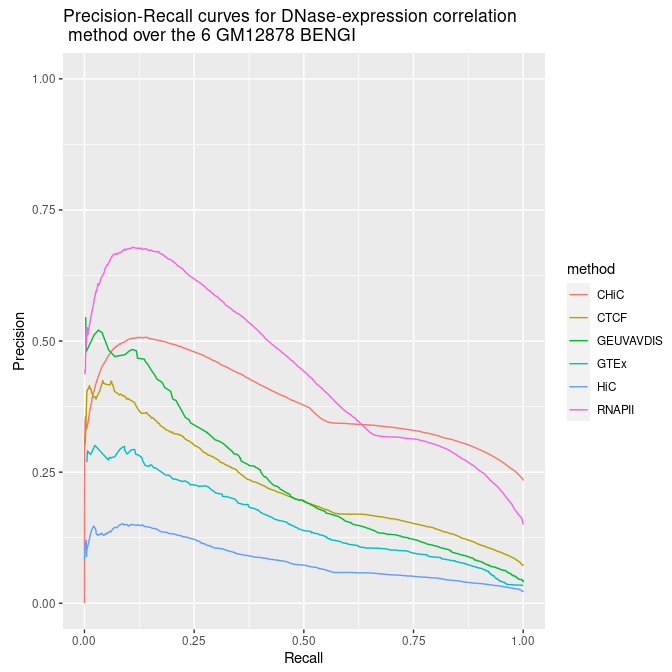
Alternatively we can plots all Precision - Recall curves on the same graph.

all_sscurves_avg_rank <- sapply(sscurves_avg_rank, simplify = FALSE, function(obj){
  Df <- data.frame(obj$prcs[[1]]$x, obj$prcs[[1]]$y)
  names(Df) <- c('x', 'y')
  return(Df)
})
all_sscurves_avg_rank <- bind_rows(all_sscurves_avg_rank, .id = 'method')

total_nrow = nrow(all_sscurves_avg_rank)
max_nb_points_to_plot = 20000
if(total_nrow>max_nb_points_to_plot){
  set.seed(1)
  samples_points = sample(1:total_nrow, min(max_nb_points_to_plot, total_nrow), replace=TRUE)
} else{
  samples_points = 1:total_nrow
}


ggplot(aes(y = y, x = x, color = method), data = all_sscurves_avg_rank[samples_points,]) + geom_line() + ylim(0,1) + xlab('Recall') + ylab('Precision') + ggtitle("Precision-Recall curves for DNase-expression correlation\n method over the 6 GM12878 BENGI")

Results¶

One can also directly have a look at the summarized results here

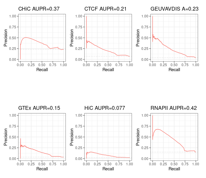
Not correcting the error in `Run-Average-Rank.sh` gives same results as in the paper¶

If we keep the small mistake found in Run-Average-Rank.sh, we find (hopefully!) the very same Precision - Recall curves as authors:

Image: Precision-Recall curves and AUPR with small mistake in Run-Average-Rank.sh

Correct results¶

If we correct the small error found in Run-Average-Rank.sh, we obtain the following results.

Image: Precision-Recall curves and AUPR

Image: Precision-Recall curves